Attractors in neural network maps: chaos and beauty

Neural networks can be thought of as dynamical systems that evolve over time in response to input data and optimization process. Attractors are a key concept in the study of dynamical systems that describe the long-term behavior of a system as it evolves towards equilibrium. In the context of neural networks, attractors can help us visualize how the network's internal representations evolve over time and converge to stable (or chaotic) states.

In this post, I explore the concept of attractors in a simple neural network that is engineered as a feedback map, and discover a range of attractors, from limit cycles to toroidal and strange attractors. This project is largely inspired by the work of J.C. Sprott "Artificial Neural Net Attractors" [1].

Setup

The example network consists of an array of input values , a hidden layer of neuron units , and output :

where are the weights and biases, and is a scaling factor. Hyperbolic tangent here plays a role of a squashing function, i.e. mapping everything to the [-1,1] interval.

Now, we can take the weights of the system as random and fixed, and we will feed the output vector to one of the input vectors at a time, so thatIt is known that such feedback systems (nonlinear maps) can exhibit chaotic behavior. Hyperparameters and weights + biases define the time-series evolution of the system, and some sets of parameters lead to the phase space settling into a basin of attraction. These attractors might be point attractors, limit cycles, toroidal and strange (chaotic) attractors.

In order to investigate how prone the system is to chaos, we will calculate the Lyapunov exponents for different sets of parameters. Lyapunov exponent is a measure of the instability of a dynamical system:where is a number of time steps, is a distance between the states and at a point in time. For stable systems converging to a fixed point or a stable attractor this parameter is less than 0, for unstable (diverging, and, therefore, chaotic systems) it is greater than 0.

The algorithm to calculate the Lyapunov exponent is as follows:

Results

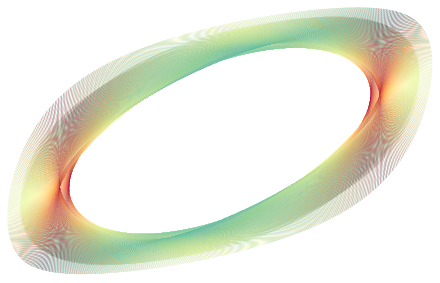
One of the stable types of attractors is the limit cycle attractor (parameters: ). The defining characteristics are: a single, closed loop trajectory in phase space. The orbit follows a regular, periodic path over time series. The structure is regular and well-defined, without the complex folding seen in toroidal or strange attractors. The Lyapunov exponent for this attractor () is negative, indicating stability.

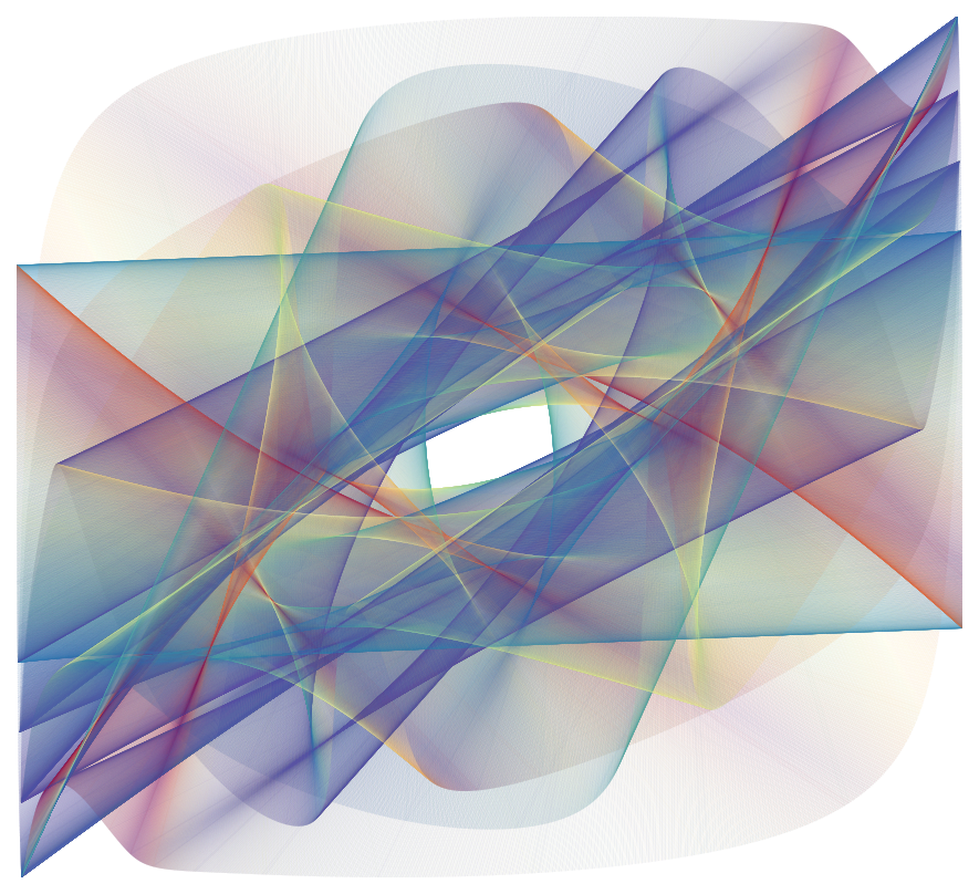
Another type of attractors is the toroidal (quasiperiodic) attractor (parameters: ). It is characterized by the ordered structure of sheets that wrap around in organized, quasiperiodic patterns. The trajectories still appear to follow predictable paths rather than the erratic, unpredictable patterns of strange attractors, while the Lyapunov exponent for this attractor approaching higher values, but is still negative ().

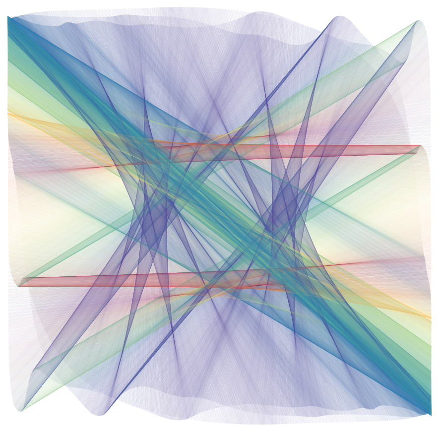
As we increase the scaling factor , the system becomes more prone to chaos. The strange (chaotic) attractor emerges with the following parameters: . It is characterized by the erratic, unpredictable patterns of trajectories that never repeat. The Lyapunov exponent for this attractor is positive (), indicating instability and chaotic behavior.

References

- J.C. Sprott, "Artificial Neural Net Attractors", Computers & Graphics, 1998. doi.org/10.1016/S0097-8493(97)00089-7